Your First Automated Trading Strategy#
In this tutorial you will be led through the creation of an automated trading strategy.
Topics Covered#
Subscribing to real time signals from a study in SC
Submitting a simple market order
Handling reversals
Using the SC trade window
Submitting attached orders
Modifying orders
Reading position information
Limiting trading to specific hours in the day
Flattening a position
Retrieving data from 2 charts (2 timeframes)
Setup#
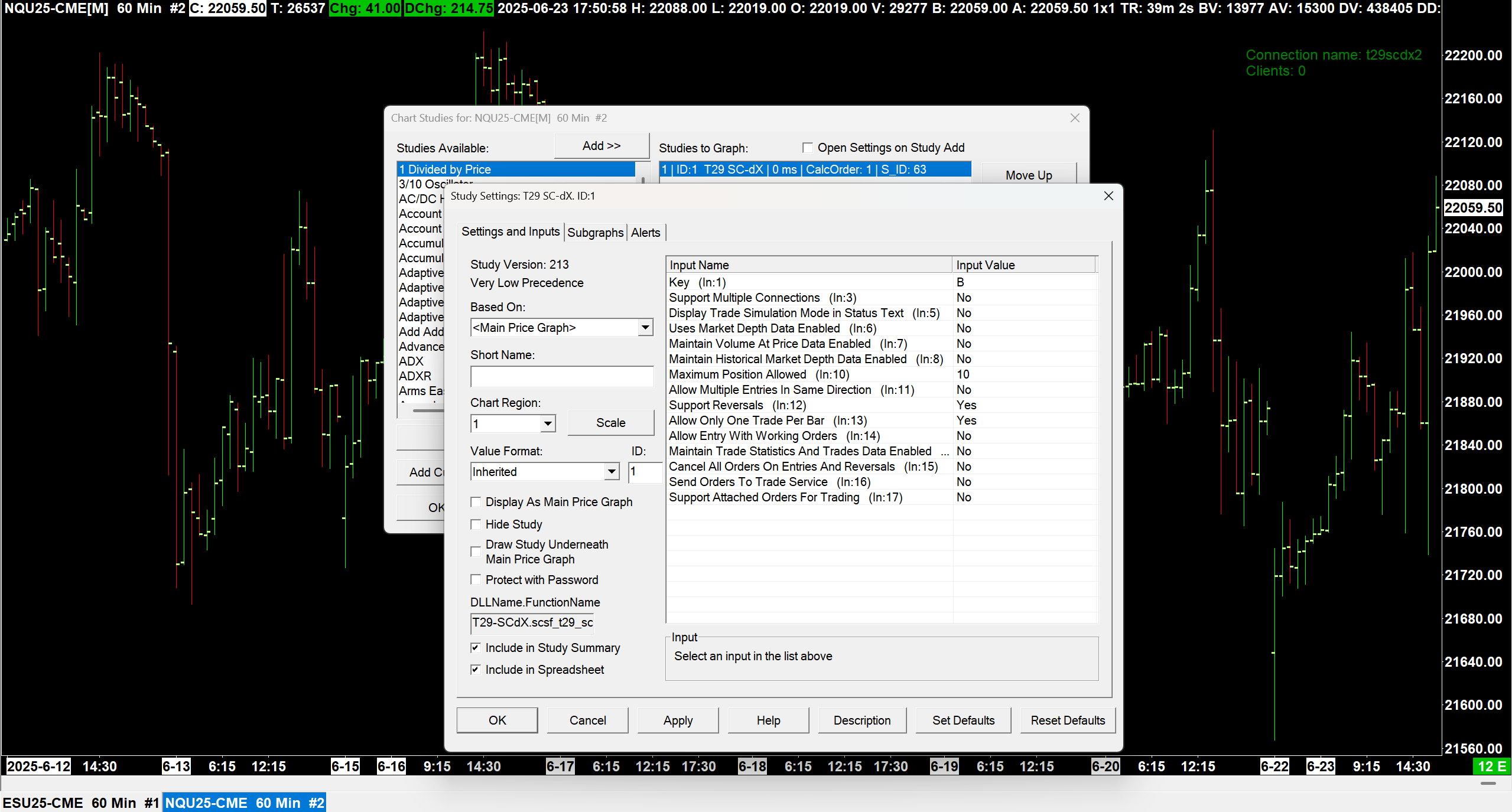
Open a 5 minute ESU24-CME chart. Add the SC-dX custom study and give the key signal. To get started we need some sort of signal to tell us when to make trades. Add the Stochastic Crossover System study to the chart and verify that you can now see buy and sell signals drawn on the chart as green and red arrows.
The Basic Strategy#
Using the signals from the stochastic crossover system, we want the following strategy:
For bearish signals:
If we are long: reverse the position
If we are short: do nothing
If we are flat: enter short
For bullish signals:
If we are long: do nothing
If we are short: reverse the position
If we are flat: enter long
Thus, once we are in the the market, with this strategy we will never exit.
Getting the Signal#
In a new python file, test that we can connect to Sierra Chart:
1from trade29.sc import SCBridge, SubgraphQuery
2
3bridge = SCBridge()
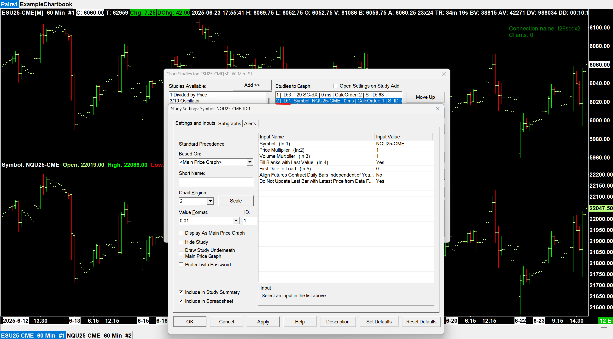
Now we want to access the signals in python. Looking at the Stochastic Crossover System study settings reveals that these signals are subgraphs with ID 1 for the buy and ID 2 for the sell subgraph.
We can subscribe to data about these subgraphs with the subscribe_to_chart_data() method.
 5subgraphs = SubgraphQuery(study_id=2, subgraphs=[1, 2])
 6
 7# Make sure to only fetch data on bar close.
 8signal_id = bridge.subscribe_to_chart_data(
 9    key='signal',
10    sg_data=[subgraphs],
11    on_bar_close=True
12)
Lets throw in some boilerplate code to print the fetched data as a dataframe to get a sense for what it looks like.
14response_queue = bridge.get_response_queue()
15
16while True:
17    response = response_queue.get()
18    print(response.as_df())
To test this we can use Sierra Chart’s replay feature. Open the replay control panel in the top bar through Chart>Replay Chart>Replay Chart (Control Panel), set the speed to something fast like 60, and scroll back through the chart (near where a signal will be given). Run the python file we just wrote, and hit Play in the Sierra Chart replay panel. We expect to see a bunch of single row DataFrames. Here is a sample output:
                     IsBarClosed  ID2.SG1  ID2.SG2
DateTime
2024-06-21 06:45:00         True      0.0      0.0
                     IsBarClosed  ID2.SG1  ID2.SG2
DateTime
2024-06-21 06:50:00         True      0.0      0.0
                     IsBarClosed  ID2.SG1  ID2.SG2
DateTime
2024-06-21 06:55:00         True      0.0      0.0
                     IsBarClosed  ID2.SG1  ID2.SG2
DateTime
2024-06-21 07:00:00         True  5542.87      0.0
                     IsBarClosed  ID2.SG1  ID2.SG2
DateTime
2024-06-21 07:05:00         True      0.0      0.0
                     IsBarClosed  ID2.SG1  ID2.SG2
DateTime
2024-06-21 07:10:00         True  5541.69      0.0
Observe how when there is no arrow drawn on the subgraph, the value is 0, and when there is, the value is the price at which it is drawn. Thus by checking if the value in this DataFrame is not 0, we can know whether we have a signal or not. So our logic would look something like this:
14response_queue = bridge.get_response_queue()
15
16while True:
17    response = response_queue.get()
18
19    buy = ...
20    sell = ...
21
22    if buy != 0:
23        # TODO: Do buying logic here
24        pass
25
26    if sell != 0:
27        # TODO: Do selling logic here
28        pass
Trading on the Signal#
Let’s start filling this in. Firstly, we need to get the actual values from the response DataFrame. Recall that SG1 was the buy signal and SG2 was the sell.
14response_queue = bridge.get_response_queue()
15
16while True:
17    response = response_queue.get()
18
19    signal_df = response.as_df(datetime_index=False, sort_datetime_ascending=False)
20
21    buy = signal_df["ID2.SG1"][0]
22    sell = signal_df["ID2.SG2"][0]
23
24    if buy != 0:
25        # TODO: Do buying logic here
26        pass
27
28    if sell != 0:
29        # TODO: Do selling logic here
30        pass
Now that we have the signals as their own variables, we can fill in the logic for what to do on a signal. Recall the outline of the strategy:
For bearish signals:
If we are long: reverse the position
If we are short: do nothing
If we are flat: enter short
For bullish signals:
If we are long: do nothing
If we are short: reverse the position
If we are flat: enter long
Given this, let position be our current position; the logic would look something like this:
14response_queue = bridge.get_response_queue()
15
16while True:
17    response = response_queue.get()
18
19    signal_df = response.as_df(datetime_index=False, sort_datetime_ascending=False)
20
21    buy = signal_df["ID2.SG1"][0]
22    sell = signal_df["ID2.SG2"][0]
23
24    position = ...
25
26    if buy != 0:
27        if position > 0: # We are long
28            pass # do nothing
29        elif position == 0: # We are flat
30            # TODO: enter long here
31            pass
32        else: # We are short
33            # TODO: reverse position here
34            pass
35
36    if sell != 0:
37        if position > 0: # We are long
38            # TODO: reverse position here
39            pass
40        elif position == 0: # We are flat
41            # TODO: enter short here
42            pass
43        else: # We are short
44            pass # do nothing
To get this position, we will add a new bridge subscription, and initialize a position variable:
 5subgraphs = SubgraphQuery(study_id=2, subgraphs=[1, 2])
 6
 7# Make sure to only fetch data on bar close.
 8signal_id = bridge.subscribe_to_chart_data(
 9    key = 'signal',
10    sg_data = [subgraphs],
11    on_bar_close = True
12)
13
14position_id = bridge.subscribe_to_position_updates(key = 'signal')
15
16position = bridge.get_position_status(key = 'signal').position_quantity
17
Now that we have two subscriptions, we need to filter the bridge response queue based on them:
19response_queue = bridge.get_response_queue()
20
21while True:
22    response = response_queue.get()
23
24    if response.request_id == position_id:
25        position = response.position_quantity
26
27    else:
28        signal_df = response.as_df(datetime_index=False, sort_datetime_ascending=False)
29
30        buy = signal_df["ID2.SG1"][0]
31        sell = signal_df["ID2.SG2"][0]
32
33        if buy != 0:
34            if position > 0: # We are long
35                pass # do nothing
36            elif position == 0: # We are flat
37                # TODO: enter long here
38                pass
39            else: # We are short
40                # TODO: reverse position here
41                pass
42
43        if sell != 0:
44            if position > 0: # We are long
45                # TODO: reverse position here
46                pass
47            elif position == 0: # We are flat
48                # TODO: enter short here
49                pass
50            else: # We are short
51                pass # do nothing
Finally, its time to fill in all of the TODOs with submit_order() calls. For this tutorial we are going to enter with a quantity of 5.
Why do we combine the cases for flat and long/short?
The submit_order() call for entering and reversing into a position is actually the same. In the SC-dX study settings SupportReversals is Yes by default. As per the Sierra Chart docs, when this option is enabled, an order that goes against the current position will first flatten the position, then execute the order. Thus to enter long and reverse into long from a short position is the same action of just buying whatever quantity you want to end up with.
19response_queue = bridge.get_response_queue()
20
21while True:
22    response = response_queue.get()
23
24    if response.request_id == position_id:
25        position = response.position_quantity
26
27    else:
28        signal_df = response.as_df(datetime_index=False, sort_datetime_ascending=False)
29
30        buy = signal_df["ID2.SG1"][0]
31        sell = signal_df["ID2.SG2"][0]
32
33        if buy != 0:
34            if position > 0: # We are long
35                pass # do nothing
36            else: # We are flat or short
37                bridge.submit_order('signal', True, 5)
38
39        if sell != 0:
40            if position >= 0: # We are flat or long
41                bridge.submit_order('signal', False, 5)
42            else: # We are short
43                pass # do nothing
Awesome! You have just finished coding your very first automated trading strategy in SC-Py. Attach the trade window to the chart under the Trade menu in the top bar, run the Python script, and replay your chart to test that the strategy works fine.
Adding Exits in Sierra Chart#
Now we are going to add a stop and a target in that SC trade window you just opened.
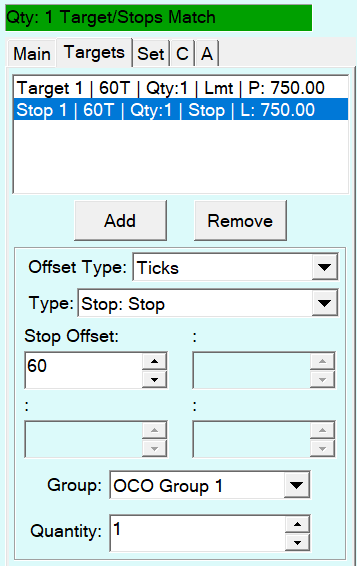
In the trade window, go to the Targets tab, and hit add to add a new target. Configure it as a limit order with an offset of 60:
Why don’t we set a quantity for attached orders?
Sierra Chart will automatically increase the quantity of the order group we defined to match the quantity of the main order we submit. Additionally, if we do set a OCO quantity in the SC Trade Window, it is expected to match the quantity under the Main tab, and will be changed if it doesn’t.
Now hit add again, and configure this order as a stop with an offset of 60. Make sure they both belong to OCO group 1.
If you tried running your python script now, you might notice that it doesn’t use these attached orders, you need to do 2 things. First in the SC Trade Window check Use Attached Orders in the Main tab, then set the attach_orders_sc_trade_window parameter in the submit_order() method:
33        if buy != 0:
34            if position > 0: # We are long
35                pass # do nothing
36            else: # We are flat or short
37                bridge.submit_order('signal', True, 5, attach_orders_sc_trade_window = True)
38
39        if sell != 0:
40            if position >= 0: # We are flat or long
41                bridge.submit_order('signal', False, 5, attach_orders_sc_trade_window = True)
42            else: # We are short
43                pass # do nothing
Now when you run you can see that a limit order and stop order are created on entrance. Awesome!
Confirming With A Trend#
We’ve come really far from our empty python file. We are now recieving a signal from a Sierra Chart study, and trading on it with stops and limits in place. This is a very strong skeleton for a trading strategy, but we can make it safer.
Using some trend indicator, we want to only enter when the direction of the signal aligns with the direction of the trend indicator. For example, suppose we get a bearish signal. If the trend is bearish too, then we can enter short, however if the trend is bullish, its safer to go flat.
Thus our logic would look something like this:
18response_queue = bridge.get_response_queue()
19
20while True:
21    response = response_queue.get()
22
23    if response.request_id == position_id:
24        position = response.position_quantity
25
26    else:
27        signal_df = response.as_df(datetime_index=False, sort_datetime_ascending=False)
28
29        trend_bearish = ...
30        trend_bullish = ...
31
32        buy = signal_df["ID2.SG1"][0]
33        sell = signal_df["ID2.SG2"][0]
34
35        if buy != 0:
36            if position > 0: # We are long
37                pass # do nothing
38            else: # We are flat or short
39                if trend_bullish:
40                    bridge.submit_order('signal', True, 5, attach_orders_sc_trade_window = True)
41                else:
42                    bridge.flatten_and_cancel('signal')
43
44        if sell != 0:
45            if position >= 0: # We are flat or long
46                if trend_bearish:
47                    bridge.submit_order('signal', False, 5, attach_orders_sc_trade_window = True)
48                else:
49                    bridge.flatten_and_cancel('signal')
50            else: # We are short
51                pass # do nothing
For the trend indicator we are going to take the slope of an exponential moving average.
In Sierra Chart, add the Moving Average - Exponential study to the chart. Note the study ID (which should be 3) and the ID of its only subgraph (SG1). Now lets add this subgraph to our chart data subscription, and lets store the trend value from one bar ago:
 5subgraphs = SubgraphQuery(study_id=2, subgraphs=[1, 2])
 6
 7trend_subgraphs = SubgraphQuery(study_id=3, subgraphs=[1])
 8
 9# Make sure to only fetch data on bar close.
10signal_id = bridge.subscribe_to_chart_data(
11    key = 'signal',
12    sg_data = [subgraphs, trend_subgraphs],
13    on_bar_close = True
14)
15
16position_id = bridge.subscribe_to_position_updates(key = 'signal')
17
18position = bridge.get_position_status(key = 'signal').position_quantity
19previous_trend_df = bridge.get_chart_data(
20    key = 'signal',
21    sg_data = [trend_subgraphs],
22    historical_bars = 1
23).as_df(datetime_index=False, sort_datetime_ascending=False)
24previous_trend = previous_trend_df["ID3.SG1"][0]
Now lets implement some logic for figuring out if our trend is bearish or bullish.
26response_queue = bridge.get_response_queue()
27
28while True:
29    response = response_queue.get()
30
31    if response.request_id == position_id:
32        position = response.position_quantity
33
34    else:
35        signal_trend_df = response.as_df(datetime_index=False, sort_datetime_ascending=False)
36
37        new_trend = signal_trend_df["ID3.SG1"][0]
38
39        if len(signal_trend_df["ID3.SG1"]) > 1:
40            # We have enough items to get a previous trend
41            previous_trend = signal_trend_df["ID3.SG1"][1]
42
43        trend_slope = new_trend - previous_trend
44
45        trend_bearish = trend_slope < 0
46        trend_bullish = trend_slope > 0
47
48        previous_trend = new_trend
49
50        buy = signal_trend_df["ID2.SG1"][0]
51        sell = signal_trend_df["ID2.SG2"][0]
A Dynamic Stop and Target#
Currently we are setting the stop and target in the Sierra Chart trade window. This was fine up until now, but our next step is going to be to set the stop and target more intelligently. Instead of having a hard set stop and target offset, we are going to dynamically set our stop and target offsets based on Sierra Chart’s Average True Range study.
Attaching Orders in Python#
Firstly, lets move the setting of the stops and targets to our python code. The submit_order() method has a parameter for OCOs, AKA attached orders. This parameter is a list of AttachedOrder . We need to add this as an import.
1from trade29.sc import SCBridge, SubgraphQuery, AttachedOrder
2
3bridge = SCBridge()
Now we need to create an attached order, and supply it to the submit_order() method.
53        target_stop = AttachedOrder(5, target_offset = 60, stop_offset = 60)
54
55        if buy != 0:
56            if position > 0: # We are long
57                pass # do nothing
58            else: # We are flat or short
59                if trend_bullish:
60                    bridge.submit_order('signal', True, 5, ocos = [target_stop])
61                else:
62                    bridge.flatten_and_cancel('signal')
63
64        if sell != 0:
65            if position >= 0: # We are flat or long
66                if trend_bearish:
67                    bridge.submit_order('signal', False, 5, ocos = [target_stop])
68                else:
69                    bridge.flatten_and_cancel('signal')
70            else: # We are short
71                pass # do nothing
Setting Offsets Dynamically#
We expect that if we run this it will have the exact same behaviour as before, as we set the exact same stops and targets in python as we had previously in Sierra Chart. Now instead of setting these stops to a constant value, lets make them dynamic.
In Sierra Chart, add the Average True Range study. Note its ID and how it only has one subgraph (the one we want) with the ID 1. Let’s add this as a subscription like we did before with our trend.
 5subgraphs = SubgraphQuery(study_id=2, subgraphs=[1, 2])
 6
 7trend_subgraphs = SubgraphQuery(study_id=3, subgraphs=[1])
 8
 9atr_subgraph = SubgraphQuery(study_id=4, subgraphs=[1])
10
11# Make sure to only fetch data on bar close.
12signal_id = bridge.subscribe_to_chart_data(
13    key = 'signal',
14    sg_data = [subgraphs, trend_subgraphs, atr_subgraph],
15    on_bar_close = True
16)
And now we can set our target and stop offsets to this ATR value!
52        buy = signal_trend_df["ID2.SG1"][0]
53        sell = signal_trend_df["ID2.SG2"][0]
54        atr = signal_trend_df["ID4.SG1"][0]
55
56        target_stop = AttachedOrder(5, target_offset = atr * 3, stop_offset = atr * 1)
57
58        if buy != 0:
59            if position > 0: # We are long
60                pass # do nothing
61            else: # We are flat or short
62                if trend_bullish:
63                    bridge.submit_order('signal', True, 5, ocos = [target_stop])
64                else:
65                    bridge.flatten_and_cancel('signal')
66
67        if sell != 0:
68            if position >= 0: # We are flat or long
69                if trend_bearish:
70                    bridge.submit_order('signal', False, 5, ocos = [target_stop])
71                else:
72                    bridge.flatten_and_cancel('signal')
73            else: # We are short
74                pass # do nothing